Simulations

pynamics.simulations

This module provides several classes for simulating dynamical systems. Both open-loop and closed-loop simulations are supported.

Classes:

Name	Description
Sim	Simulate a dynamical system and plot the results.

Sim(system, input_signal, t0=0.0, tfinal=10.0, solver='RK4', step_size=0.001, mode='open_loop', controller=None, reference_labels=None, reference_lookahead=1, noise_power=0.0, noise_seed=0)

Bases: _BaseSimulator

Simulate a dynamical system.

This class can be used to simulate the behaviour of a dynamical system. It supports both open- and closed-loop simulations, which makes it appropriate for both system analysis and control design.

Parameters:

Name	Type	Description	Default
system	BaseModel	System to simulate. Must be described by a model supported by Pynamics.	required
input_signal	ndarray	Input signals. These may be reference values or other external inputs (e.g. wind speed in a wind turbine system).	required
t0	float	Initial time instant. Must be non-negative.	0.0
tfinal	float	Final time instant. Must be non-negative.	0.0
solver	(RK4, Euler, Modified_Euler, Heun)	Fixed-step solver.	"RK4"
step_size	float	Solver step size. Must be positive.	0.001
mode	(open_loop, closed_loop)	Simulation mode. The controller will not be included in the simulation unless parameter is set to "closed_loop".	"open_loop"
controller	BaseController | None	Controller.	None
reference_labels	list[str] | None	List of labels for the reference signals.	None
reference_lookahead	int	Number of time steps ahead for which the reference values are known to the controller.	1
noise_power	int | float	White noise power. If equal to zero, no noise will be added to the simulation.	0.0
noise_seed	int	Random seed for the noise array.	0

Attributes:

Name	Type	Description
system	BaseModel	The system to simulate.
options	dict	Simulation options (initial and final time instants).
solver	_FixedStepSolver	Solver.
time	ndarray	Time array.
inputs	ndarray	The input signals.
outputs	ndarray	The output signals.
noise	ndarray	Array of white noise values.
control_actions	ndarray	Array of control actions.
controller	BaseController	Controller.
ref_lookahead	int	Number of time steps ahead for which the reference values are known to the controller.
ref_labels	list[str]	List of labels for the reference signals.

Methods:

Name	Description
summary	Display the current simulation settings.
run	Run a simulation.
reset	Reset the output and control actions arrays, as well as the system's state and input vectors, so that a new simulation can be run.
tracking_plot	Evaluate the system's tracking performance by plotting the reference signal and the system's output (SISO systems only).
system_outputs_plot	Visualise the system's output signals.
step_response	Simulate the system's step response (single-input systems or single-reference controllers only).
ramp	Simulate the system's response to a ramp signal (single-input systems or single-reference controllers only).

Raises:

Type	Description
TypeError	If a value of the wrong type is passed as a parameter.
ValueError	If the value of any parameter is invalid (e.g. input signal has the wrong length, mode is neither "open_loop" nor "closed_loop", etc.).

Warning

Only fixed-step solvers are support at the moment.

Source code in pynamics/simulations.py

def __init__(self, 
             system: BaseModel, 
             input_signal: np.ndarray, 
             t0: float=0.0, 
             tfinal: float=10.0, 
             solver: str="RK4", 
             step_size: float=0.001, 
             mode: str="open_loop", 
             controller: BaseController | None=None, 
             reference_labels: list[str] | None=None, 
             reference_lookahead: int=1, 
             noise_power: int | float=0.0, 
             noise_seed: int=0) -> None:
    """
    Class constructor.
    """

    super().__init__(system, t0, tfinal, solver, step_size);
    self._mode_check(mode);
    self._mode = mode;
    self._input_checks(input_signal);
    self._inputs = self._input_reformatting(input_signal);
    self.outputs = np.zeros(shape=(self.system.output_dim, self.time.shape[0]));
    self.noise = _white_noise(self.system.output_dim, self.time.shape[0], noise_power, noise_seed);
    self._lookahead_check(reference_lookahead);
    self._ref_lookahead = reference_lookahead;
    self.controller = controller;

    if(self._mode == "open_loop"):

        self.controller = DummyController(self.inputs.shape[0], self.system.input_dim, step_size);

    self.control_actions = np.zeros(shape=(self.controller.output_dim, self.time.shape[0]));
    self.ref_labels = self._labels_check(reference_labels);

    return;

inputs: np.ndarray property writable

Get the input signals.

This method can be used to access the input / reference signals using dot notation.

Returns:

Type	Description
ndarray	System input signals.

ref_lookahead: int property writable

Get the ref_lookahead parameter.

This method can be used to access the value of the ref_lookahead parameter using dot notation.

Returns:

Type	Description
int	Number of time steps ahead for which the reference values are known to the controller.

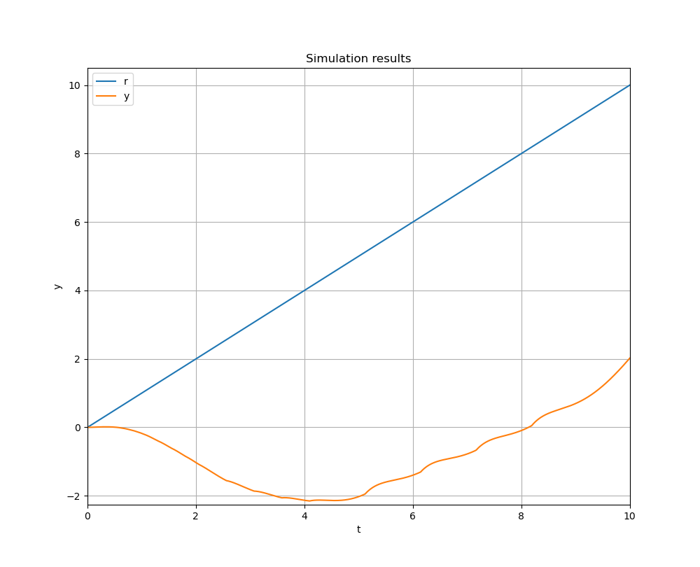
ramp(system, slope=1.0, t0=0.0, tfinal=10.0, solver='RK4', step_size=0.001, mode='open_loop', controller=None, reference_labels=None, reference_lookahead=1, noise_power=0.0, noise_seed=0) classmethod

Simulate the system's response to a ramp signal.

This method can be used to simulate a system's response to a ramp input. Keep in mind that, for now, it should only be used with single-input systems or controllers needing only one reference signal.

Parameters:

Name	Type	Description	Default
system	BaseModel	System to simulate. Must be described by a model supported by Pynamics.	required
slope	int | float	The ramp's slope. Unit ramp by default.	1.0
t0	float	Initial time instant. Must be non-negative.	0.0
tfinal	float	Final time instant. Must be non-negative.	0.0
solver	(RK4, Euler, Modified_Euler, Heun)	Fixed-step solver.	"RK4"
step_size	float	Solver step size. Must be positive.	0.001
mode	(open_loop, closed_loop)	Simulation mode. The controller will not be included in the simulation unless parameter is set to "closed_loop".	"open_loop"
controller	BaseController | None	Controller.	None
reference_labels	list[str] | None	List of labels for the reference signals.	None
reference_lookahead	int	Number of time steps ahead for which the reference values are known to the controller.	1
noise_power	int | float	White noise power. If equal to zero, no noise will be added to the simulation.	0.0
noise_seed	int	Random seed for the noise array.	0

Returns:

Type	Description
Sim	A simulation class instance.

Warning

It seems this method might be somewhat inaccurate at the moment. Results might not be as reliable.

Examples:

>>> import numpy as np
>>> from pynamics.models.state_space_models import LinearModel
>>> from pynamics.simulations import Sim
>>> 
>>> A = np.array([[0, 0, -1], [1, 0, -3], [0, 1, -3]]);
>>> B = np.array([1, -5, 1]).reshape(-1, 1);
>>> C = np.array([0, 0, 1]);
>>> D = np.array([0]);
>>> model = LinearModel(np.zeros((3, 1)), np.zeros((1, 1)), A, B, C, D);
>>>
>>> simulation = Sim.ramp(model, slope=1);
>>> res = simulation.run();
>>> 
>>> _ = Sim.tracking_plot(res, "Time", "Ref_1", "y_1");

Source code in pynamics/simulations.py

@classmethod
def ramp(cls,
         system: BaseModel, 
         slope: int | float=1.0, 
         t0: float=0.0, 
         tfinal: float=10.0, 
         solver: str="RK4", 
         step_size: float=0.001, 
         mode: str="open_loop", 
         controller: any=None, 
         reference_labels: list[str] | None=None, 
         reference_lookahead: int=1, \
         noise_power: int | float=0.0, 
         noise_seed: int=0):
    """
    Simulate the system's response to a ramp signal.

    This method can be used to simulate a system's response to a ramp input. Keep in mind that, for now, it should only be used \
    with single-input systems or controllers needing only one reference signal.

    Parameters
    ----------
    system : BaseModel
        System to simulate. Must be described by a model supported by [Pynamics](../index.md).

    slope : int | float, default=1.0
        The ramp's slope. Unit ramp by default.

    t0 : float, default=0.0
        Initial time instant. Must be non-negative.

    tfinal : float, default=0.0
        Final time instant. Must be non-negative.

    solver : {"RK4", "Euler", "Modified_Euler", "Heun"}, str, default="RK4"
        Fixed-step solver.

    step_size : float, default=0.001
        Solver step size. Must be positive.

    mode : {"open_loop", "closed_loop"}, str, default="open_loop"
        Simulation mode. The controller will not be included in the simulation unless \
        parameter is set to "closed_loop".

    controller : BaseController | None, optional
        Controller.

    reference_labels : list[str] | None, optional
        List of labels for the reference signals.

    reference_lookahead : int, default=1
        Number of time steps ahead for which the reference values are known to the controller.

    noise_power : int | float, default=0.0
        White noise power. If equal to zero, no noise will be added to the simulation.

    noise_seed : int, default=0
        Random seed for the noise array.

    Returns
    -------
    Sim
        A simulation class instance.

    Warning
    -------
    It seems this method might be somewhat inaccurate at the moment. Results might not be as reliable.

    Examples
    --------
    >>> import numpy as np
    >>> from pynamics.models.state_space_models import LinearModel
    >>> from pynamics.simulations import Sim
    >>> 
    >>> A = np.array([[0, 0, -1], [1, 0, -3], [0, 1, -3]]);
    >>> B = np.array([1, -5, 1]).reshape(-1, 1);
    >>> C = np.array([0, 0, 1]);
    >>> D = np.array([0]);
    >>> model = LinearModel(np.zeros((3, 1)), np.zeros((1, 1)), A, B, C, D);
    >>>
    >>> simulation = Sim.ramp(model, slope=1);
    >>> res = simulation.run();
    >>> 
    >>> _ = Sim.tracking_plot(res, "Time", "Ref_1", "y_1");

    ![Ramp_img](../images/Ramp_fig.png)
    """

    reference_signal = slope * np.arange(t0, tfinal + step_size, step_size);

    return cls(system, 
               reference_signal, 
               t0, 
               tfinal, 
               solver, 
               step_size, 
               mode, 
               controller, 
               reference_labels, 
               reference_lookahead, 
               noise_power, 
               noise_seed);

reset(initial_state, initial_control)

Reset simulation parameters (initial conditions, output arrays, control actions).

This method must be called every time one wishes to run another simulation. The initial conditions, output array and control actions array are all reset. This method is useful if one wishes to run simulations with different initial conditions or different controllers.

Parameters:

Name	Type	Description	Default
initial_state	ndarray	The system's initial state. Should be an array shaped (n, 1), where n is the number of state variables.	required
initial_control	ndarray | float	The inputs' initial value(s). Should be an array shaped (u, 1), where u is the number of input variables.	required

Examples:

>>> import numpy as np
>>> from pynamics.models.state_space_models import LinearModel
>>> from pynamics.simulations import Sim
>>> 
>>> A = np.array([[0, 0, -1], [1, 0, -3], [0, 1, -3]]);
>>> B = np.array([1, -5, 1]).reshape(-1, 1);
>>> C = np.array([0, 0, 1]);
>>> D = np.array([0]);
>>> model = LinearModel(np.zeros((3, 1)), np.zeros((1, 1)), A, B, C, D);
>>>
>>> simulation = Sim(model, input_signal=np.ones(int(10/0.001)+1));
>>> res = simulation.run();
>>> simulation.system.x
array([[7.98056883],
       [1.96495125],
       [0.98406462]])
>>>
>>> simulation.reset(np.zeros((3, 1)), np.zeros((1, 1)));
Sim outputs and control actions were reset sucessfully.
>>> simulation.system.x
array([[0.],
       [0.],
       [0.]])

Source code in pynamics/simulations.py

def reset(self, initial_state: np.ndarray, initial_control: np.ndarray | float) -> None:
    """
    Reset simulation parameters (initial conditions, output arrays, control actions).

    This method must be called every time one wishes to run another simulation. The initial conditions, \
    output array and control actions array are all reset. This method is useful if one wishes to run \
    simulations with different initial conditions or different controllers.

    Parameters
    ----------
    initial_state : np.ndarray
        The system's initial state. Should be an array shaped (n, 1), where n \
        is the number of state variables.

    initial_control: np.ndarray
        The inputs' initial value(s). Should be an array shaped (u, 1), where
        u is the number of input variables.

    Examples
    --------
    >>> import numpy as np
    >>> from pynamics.models.state_space_models import LinearModel
    >>> from pynamics.simulations import Sim
    >>> 
    >>> A = np.array([[0, 0, -1], [1, 0, -3], [0, 1, -3]]);
    >>> B = np.array([1, -5, 1]).reshape(-1, 1);
    >>> C = np.array([0, 0, 1]);
    >>> D = np.array([0]);
    >>> model = LinearModel(np.zeros((3, 1)), np.zeros((1, 1)), A, B, C, D);
    >>>
    >>> simulation = Sim(model, input_signal=np.ones(int(10/0.001)+1));
    >>> res = simulation.run();
    >>> simulation.system.x
    array([[7.98056883],
           [1.96495125],
           [0.98406462]])
    >>>
    >>> simulation.reset(np.zeros((3, 1)), np.zeros((1, 1)));
    Sim outputs and control actions were reset sucessfully.
    >>> simulation.system.x
    array([[0.],
           [0.],
           [0.]])
    """

    self.system.x = initial_state;
    self.system.set_input(initial_control);
    self.outputs = np.zeros(shape=(self.system.output_dim, self.time.shape[0]));
    self.control_actions = np.zeros(shape=(self.controller.output_dim, self.time.shape[0]));
    print("Sim outputs and control actions were reset sucessfully.");

    return;

run()

Run a simulation.

This method is used to run a simulation.

Returns:

Type	Description
DataFrame	Data frame containing the results.

Examples:

>>> import numpy as np
>>> from pynamics.models.state_space_models import LinearModel
>>> from pynamics.simulations import Sim
>>> 
>>> A = np.array([[0, 0, -1], [1, 0, -3], [0, 1, -3]]);
>>> B = np.array([1, -5, 1]).reshape(-1, 1);
>>> C = np.array([0, 0, 1]);
>>> D = np.array([0]);
>>> model = LinearModel(np.zeros((3, 1)), np.zeros((1, 1)), A, B, C, D);
>>>
>>> simulation = Sim(model, input_signal=np.ones(int(10/0.001)+1));
>>> res = simulation.run();
>>> res
         Time  Ref_1  u_1       y_1
0       0.000    1.0  0.0  0.000000
1       0.001    1.0  1.0  0.000996
2       0.002    1.0  1.0  0.001984
3       0.003    1.0  1.0  0.002964
4       0.004    1.0  1.0  0.003936
...       ...    ...  ...       ...
9996    9.996    1.0  1.0  0.984014
9997    9.997    1.0  1.0  0.984026
9998    9.998    1.0  1.0  0.984039
9999    9.999    1.0  1.0  0.984052
10000  10.000    1.0  1.0  0.984065

[10001 rows x 4 columns]

Source code in pynamics/simulations.py

def run(self) -> pd.DataFrame:     
    """
    Run a simulation.

    This method is used to run a simulation.

    Returns
    -------
    pd.DataFrame
        Data frame containing the results.

    Examples
    --------
    >>> import numpy as np
    >>> from pynamics.models.state_space_models import LinearModel
    >>> from pynamics.simulations import Sim
    >>> 
    >>> A = np.array([[0, 0, -1], [1, 0, -3], [0, 1, -3]]);
    >>> B = np.array([1, -5, 1]).reshape(-1, 1);
    >>> C = np.array([0, 0, 1]);
    >>> D = np.array([0]);
    >>> model = LinearModel(np.zeros((3, 1)), np.zeros((1, 1)), A, B, C, D);
    >>>
    >>> simulation = Sim(model, input_signal=np.ones(int(10/0.001)+1));
    >>> res = simulation.run();
    >>> res
             Time  Ref_1  u_1       y_1
    0       0.000    1.0  0.0  0.000000
    1       0.001    1.0  1.0  0.000996
    2       0.002    1.0  1.0  0.001984
    3       0.003    1.0  1.0  0.002964
    4       0.004    1.0  1.0  0.003936
    ...       ...    ...  ...       ...
    9996    9.996    1.0  1.0  0.984014
    9997    9.997    1.0  1.0  0.984026
    9998    9.998    1.0  1.0  0.984039
    9999    9.999    1.0  1.0  0.984052
    10000  10.000    1.0  1.0  0.984065
    <BLANKLINE>
    [10001 rows x 4 columns]
    """

    self.control_actions[:, 0] = self.system.get_input();
    self.outputs[:, 0] = self.system.get_output();

    #for ind, (t, _, y, n, _) in enumerate(zip(self.time[:-1], self.inputs[:, :-1], self.outputs[:, :-1], self.noise[:, :-1], self.control_actions[:, :-1])):
    for ind, t in enumerate(self.time[:-1]):

        #self.outputs[:, ind+1], self.control_actions[:, ind+1] = self._step(t, ref, y + n);
        self.outputs[:, ind+1], self.control_actions[:, ind+1] = self._step(t, self.inputs[:, ind:ind+self.ref_lookahead], self.outputs[:, ind:ind+1]); # + self.noise[:, ind:ind+1]
        #self.outputs[:, ind+1], self.control_actions[:, ind+1] = self._step(t, self.inputs[:, ind:ind+self.ref_lookahead], y + n);
        self.outputs[:, ind+1] += self.noise[:, ind+1];

    # Create results data frame
    names = ["Time"];
    names.extend(self.ref_labels);
    names.extend(self.system.input_labels);
    names.extend(self.system.output_labels);

    results = np.expand_dims(self.time, axis=0).T;
    results = np.hstack((results, self.inputs.T));
    results = np.hstack((results, self.control_actions.T));
    results = np.hstack((results, self.outputs.T));

    sim_data = pd.DataFrame(results, columns=names);

    return sim_data;

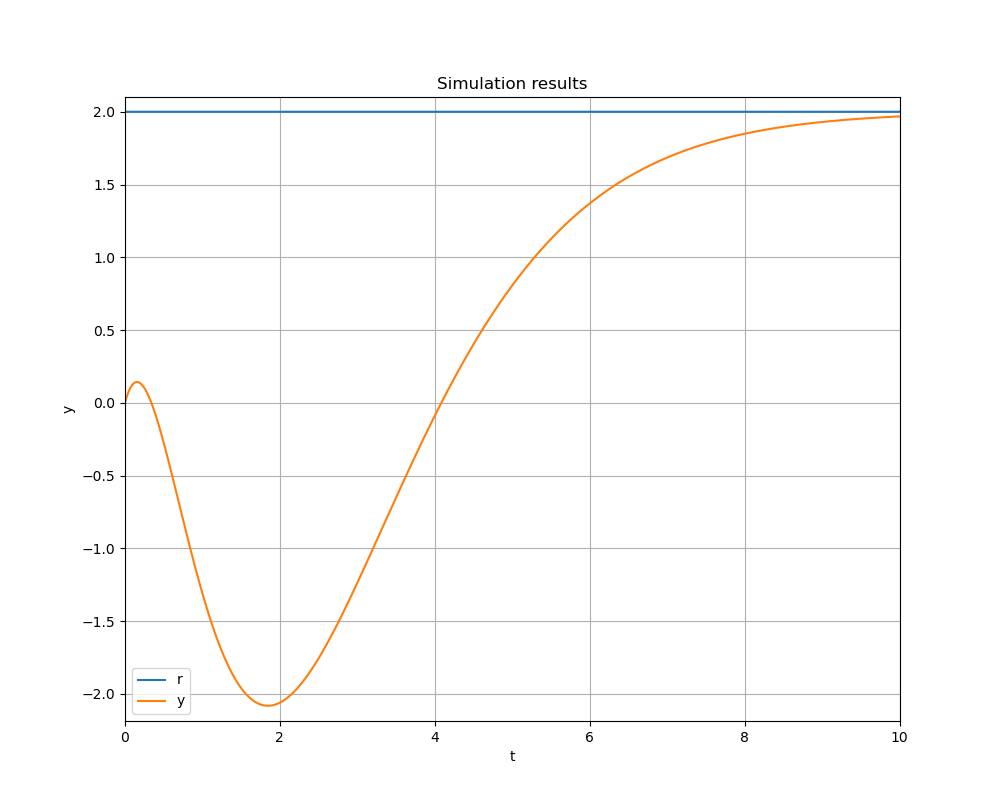
step_response(system, step_magnitude=1.0, t0=0.0, tfinal=10.0, solver='RK4', step_size=0.001, mode='open_loop', controller=None, reference_labels=None, reference_lookahead=1, noise_power=0.0, noise_seed=0) classmethod

Simulate the step response of a dynamical system.

This method can be used to simulate a system's step response. Keep in mind that, for now, it should only be used with single-input systems or controllers needing only one reference signal.

Parameters:

Name	Type	Description	Default
system	BaseModel	System to simulate. Must be described by a model supported by Pynamics.	required
step_magnitude	int | float	The step's magnitude. Unit step by default.	1.0
t0	float	Initial time instant. Must be non-negative.	0.0
tfinal	float	Final time instant. Must be non-negative.	0.0
solver	(RK4, Euler, Modified_Euler, Heun)	Fixed-step solver.	"RK4"
step_size	float	Solver step size. Must be positive.	0.001
mode	(open_loop, closed_loop)	Simulation mode. The controller will not be included in the simulation unless parameter is set to "closed_loop".	"open_loop"
controller	BaseController | None	Controller.	None
reference_labels	list[str] | None	List of labels for the reference signals.	None
reference_lookahead	int	Number of time steps ahead for which the reference values are known to the controller.	1
noise_power	int | float	White noise power. If equal to zero, no noise will be added to the simulation.	0.0
noise_seed	int	Random seed for the noise array.	0

Returns:

Type	Description
Sim	A simulation class instance.

Examples:

>>> import numpy as np
>>> from pynamics.models.state_space_models import LinearModel
>>> from pynamics.simulations import Sim
>>> 
>>> A = np.array([[0, 0, -1], [1, 0, -3], [0, 1, -3]]);
>>> B = np.array([1, -5, 1]).reshape(-1, 1);
>>> C = np.array([0, 0, 1]);
>>> D = np.array([0]);
>>> model = LinearModel(np.zeros((3, 1)), np.zeros((1, 1)), A, B, C, D);
>>>
>>> simulation = Sim.step_response(model, step_magnitude=2);
>>> res = simulation.run();
>>> 
>>> _ = Sim.tracking_plot(res, "Time", "Ref_1", "y_1");

Source code in pynamics/simulations.py

@classmethod
def step_response(cls,
                  system: BaseModel, 
                  step_magnitude: int | float=1.0, 
                  t0: float=0.0, 
                  tfinal: float=10.0, 
                  solver: str="RK4", 
                  step_size: float=0.001, 
                  mode: str="open_loop", 
                  controller: any=None, 
                  reference_labels: list[str] | None=None, 
                  reference_lookahead: int=1, \
                  noise_power: int | float=0.0, 
                  noise_seed: int=0):
    """
    Simulate the step response of a dynamical system.

    This method can be used to simulate a system's step response. Keep in mind that, for now, it should only be used \
    with single-input systems or controllers needing only one reference signal.

    Parameters
    ----------
    system : BaseModel
        System to simulate. Must be described by a model supported by [Pynamics](../index.md).

    step_magnitude : int | float, default=1.0
        The step's magnitude. Unit step by default.

    t0 : float, default=0.0
        Initial time instant. Must be non-negative.

    tfinal : float, default=0.0
        Final time instant. Must be non-negative.

    solver : {"RK4", "Euler", "Modified_Euler", "Heun"}, str, default="RK4"
        Fixed-step solver.

    step_size : float, default=0.001
        Solver step size. Must be positive.

    mode : {"open_loop", "closed_loop"}, str, default="open_loop"
        Simulation mode. The controller will not be included in the simulation unless \
        parameter is set to "closed_loop".

    controller : BaseController | None, optional
        Controller.

    reference_labels : list[str] | None, optional
        List of labels for the reference signals.

    reference_lookahead : int, default=1
        Number of time steps ahead for which the reference values are known to the controller.

    noise_power : int | float, default=0.0
        White noise power. If equal to zero, no noise will be added to the simulation.

    noise_seed : int, default=0
        Random seed for the noise array.

    Returns
    -------
    Sim
        A simulation class instance.

    Examples
    --------
    >>> import numpy as np
    >>> from pynamics.models.state_space_models import LinearModel
    >>> from pynamics.simulations import Sim
    >>> 
    >>> A = np.array([[0, 0, -1], [1, 0, -3], [0, 1, -3]]);
    >>> B = np.array([1, -5, 1]).reshape(-1, 1);
    >>> C = np.array([0, 0, 1]);
    >>> D = np.array([0]);
    >>> model = LinearModel(np.zeros((3, 1)), np.zeros((1, 1)), A, B, C, D);
    >>>
    >>> simulation = Sim.step_response(model, step_magnitude=2);
    >>> res = simulation.run();
    >>> 
    >>> _ = Sim.tracking_plot(res, "Time", "Ref_1", "y_1");

    ![Step_response_img](../images/Step_response_fig.png)
    """

    end = (tfinal - t0) / step_size + 1;
    reference_signal = np.full(shape=(1, int(end)), fill_value=step_magnitude);

    return cls(system, 
               reference_signal, 
               t0, 
               tfinal, 
               solver, 
               step_size, 
               mode, 
               controller, 
               reference_labels, 
               reference_lookahead, 
               noise_power, 
               noise_seed);

summary()

Display the current simulation settings.

This method displays the value of the most important simulation options.

Examples:

>>> import numpy as np
>>> from pynamics.models.state_space_models import LinearModel
>>> from pynamics.simulations import Sim
>>> 
>>> A = np.array([[0, 0, -1], [1, 0, -3], [0, 1, -3]]);
>>> B = np.array([1, -5, 1]).reshape(-1, 1);
>>> C = np.array([0, 0, 1]);
>>> D = np.array([0]);
>>> model = LinearModel(np.zeros((3, 1)), np.zeros((1, 1)), A, B, C, D);
>>>
>>> simulation = Sim(model, input_signal=np.ones(int(10/0.001)+1));
>>> simulation.summary();
Simulation settings
-------------------
Initial time step: 0.0 s
Final time step: 10.0 s
Solver step size: 0.001 s
-------------------
Input signals format: (1, 10001)
Output signals format: (1, 10001)
Control actions format: (1, 10001)
Reference lookahead: 1 time step
-------------------
Simulation mode: open_loop

Source code in pynamics/simulations.py

def summary(self) -> None:
    """
    Display the current simulation settings.

    This method displays the value of the most important simulation options.

    Examples
    --------
    >>> import numpy as np
    >>> from pynamics.models.state_space_models import LinearModel
    >>> from pynamics.simulations import Sim
    >>> 
    >>> A = np.array([[0, 0, -1], [1, 0, -3], [0, 1, -3]]);
    >>> B = np.array([1, -5, 1]).reshape(-1, 1);
    >>> C = np.array([0, 0, 1]);
    >>> D = np.array([0]);
    >>> model = LinearModel(np.zeros((3, 1)), np.zeros((1, 1)), A, B, C, D);
    >>>
    >>> simulation = Sim(model, input_signal=np.ones(int(10/0.001)+1));
    >>> simulation.summary();
    Simulation settings
    -------------------
    Initial time step: 0.0 s
    Final time step: 10.0 s
    Solver step size: 0.001 s
    -------------------
    Input signals format: (1, 10001)
    Output signals format: (1, 10001)
    Control actions format: (1, 10001)
    Reference lookahead: 1 time step
    -------------------
    Simulation mode: open_loop
    """

    print("Simulation settings");
    print("-------------------");
    print(f"Initial time step: {self._options["t0"]} s");
    print(f"Final time step: {self._options["tfinal"]} s");
    print(f"Solver step size: {self._solver.h} s");
    #print(f"Solver: {self._solver}");
    print("-------------------");
    print(f"Input signals format: {self._inputs.shape}");
    print(f"Output signals format: {self.outputs.shape}");
    print(f"Control actions format: {self.control_actions.shape}");
    print(f"Reference lookahead: {self._ref_lookahead} time step");
    print("-------------------");
    print(f"Simulation mode: {self._mode}");
    #print(f"Controller: {self.controller}");

    return;

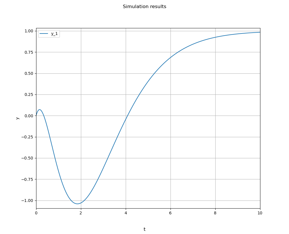
system_outputs_plot(sim_results, time_variable, outputs, plot_title='Simulation results', xlabel='t', ylabel='y', plot_height=10.0, plot_width=10.0) staticmethod

Visualise the system's output signals.

This method can be use to visualise the system's output signals simultaneously. It supports MIMO systems.

Parameters:

Name	Type	Description	Default
sim_results	DataFrame	Simulation results.	required
time_variable	str	Name of the time variable.	required
outputs	list[str]	List containing the names of the output variables.	required
plot_title	str	Plot title.	"Simulation results"
xlabel	str	X-axis label.	"t"
ylabel	str	Y-axis label	"y"
plot_height	int | float	Figure height.	10.0
plot_width	int | float	Figure width.	10.0

Examples:

>>> import numpy as np
>>> from pynamics.models.state_space_models import LinearModel
>>> from pynamics.simulations import Sim
>>> 
>>> A = np.array([[0, 0, -1], [1, 0, -3], [0, 1, -3]]);
>>> B = np.array([1, -5, 1]).reshape(-1, 1);
>>> C = np.array([0, 0, 1]);
>>> D = np.array([0]);
>>> model = LinearModel(np.zeros((3, 1)), np.zeros((1, 1)), A, B, C, D);
>>>
>>> simulation = Sim(model, input_signal=np.ones(int(10/0.001)+1));
>>> res = simulation.run();
>>> 
>>> _ = Sim.system_outputs_plot(res, "Time", ["y_1"]);

Source code in pynamics/simulations.py

@staticmethod
def system_outputs_plot(sim_results: pd.DataFrame,
                        time_variable: str,
                        outputs: list[str], 
                        plot_title: str="Simulation results", 
                        xlabel: str="t", 
                        ylabel: str="y", 
                        plot_height: int | float=10.0, 
                        plot_width: int | float=10.0) -> None:
    """
    Visualise the system's output signals.

    This method can be use to visualise the system's output signals simultaneously. \
    It supports MIMO systems.

    Parameters
    ----------
    sim_results : pd.DataFrame
        Simulation results.

    time_variable : str
        Name of the time variable.

    outputs : list[str]
        List containing the names of the output variables.

    plot_title : str, default="Simulation results"
        Plot title.

    xlabel : str, default="t"
        X-axis label.

    ylabel : str, default="y"
        Y-axis label

    plot_height : int | float, default=10.0
        Figure height.

    plot_width : int | float, default=10.0
        Figure width.

    Examples
    --------
    >>> import numpy as np
    >>> from pynamics.models.state_space_models import LinearModel
    >>> from pynamics.simulations import Sim
    >>> 
    >>> A = np.array([[0, 0, -1], [1, 0, -3], [0, 1, -3]]);
    >>> B = np.array([1, -5, 1]).reshape(-1, 1);
    >>> C = np.array([0, 0, 1]);
    >>> D = np.array([0]);
    >>> model = LinearModel(np.zeros((3, 1)), np.zeros((1, 1)), A, B, C, D);
    >>>
    >>> simulation = Sim(model, input_signal=np.ones(int(10/0.001)+1));
    >>> res = simulation.run();
    >>> 
    >>> _ = Sim.system_outputs_plot(res, "Time", ["y_1"]);

    ![System_outputs_img](../images/Outputs_plot_fig.png)
    """

    fig, axes = plt.subplots(len(outputs), 1, sharex=True);
    fig.set_figheight(plot_height);
    fig.set_figwidth(plot_width);
    fig.suptitle(plot_title);
    fig.supxlabel(xlabel);
    xfactor = 1.0005;
    yfactor = 1.05;

    if (len(outputs) > 1):

        for it, (_, output) in enumerate(zip(axes, outputs)):

            axes[it].plot(sim_results[time_variable], sim_results[output], label=output);
            axes[it].set_ylabel(ylabel);
            axes[it].grid(visible=True);
            axes[it].legend();
            axes[it].set_xlim([sim_results[time_variable].min() * xfactor, sim_results[time_variable].max() * xfactor]);
            axes[it].set_ylim([sim_results[output].min() * yfactor, sim_results[output].max() * yfactor]);

    else:

        axes.plot(sim_results[time_variable], sim_results[outputs[0]], label=outputs[0]);
        axes.set_ylabel(ylabel);
        axes.grid(visible=True);
        axes.legend();
        axes.set_xlim([sim_results[time_variable].min() * xfactor, sim_results[time_variable].max() * xfactor]);
        axes.set_ylim([sim_results[outputs[0]].min() * yfactor, sim_results[outputs[0]].max() * yfactor]); 

    plt.show();

    return;

tracking_plot(sim_results, time_variable, reference, output, plot_title='Simulation results', xlabel='t', ylabel='y', plot_height=10.0, plot_width=10.0) staticmethod

Plot the reference signal and the system's output.

Evaluate the system's tracking performance by plotting the reference signal and the system's output (SISO systems only).

Parameters:

Name	Type	Description	Default
sim_results	DataFrame	Simulation results.	required
time_variable	str	Name of the time variable.	required
reference	str	Name of the reference variable.	required
output	str	Name of the output variable.	required
plot_title	str	Plot title.	"Simulation results"
xlabel	str	X-axis label.	"t"
ylabel	str	Y-axis label.	"y"
plot_height	int | float	Figure height.	10.0
plot_width	int | float	Figure width.	10.0

Examples:

>>> import numpy as np
>>> from pynamics.models.state_space_models import LinearModel
>>> from pynamics.simulations import Sim
>>> 
>>> A = np.array([[0, 0, -1], [1, 0, -3], [0, 1, -3]]);
>>> B = np.array([1, -5, 1]).reshape(-1, 1);
>>> C = np.array([0, 0, 1]);
>>> D = np.array([0]);
>>> model = LinearModel(np.zeros((3, 1)), np.zeros((1, 1)), A, B, C, D);
>>>
>>> simulation = Sim(model, input_signal=np.ones(int(10/0.001)+1));
>>> res = simulation.run();
>>> 
>>> _ = Sim.tracking_plot(res, "Time", "Ref_1", "y_1");

Source code in pynamics/simulations.py

@staticmethod
def tracking_plot(sim_results: pd.DataFrame,
                  time_variable: str,
                  reference: str,
                  output: str, 
                  plot_title: str="Simulation results", 
                  xlabel: str="t", 
                  ylabel: str="y", 
                  plot_height: int | float=10.0, 
                  plot_width: int | float=10.0) -> None:
    """
    Plot the reference signal and the system's output.

    Evaluate the system's tracking performance by plotting the reference signal and the system's output (SISO systems only).

    Parameters
    ----------
    sim_results : pd.DataFrame
        Simulation results.

    time_variable : str
        Name of the time variable.

    reference : str
        Name of the reference variable.

    output : str
        Name of the output variable.

    plot_title : str, default="Simulation results"
        Plot title.

    xlabel : str, default="t"
        X-axis label.

    ylabel : str, default="y"
        Y-axis label.

    plot_height : int | float, default=10.0
        Figure height.

    plot_width : int | float, default=10.0
        Figure width.

    Examples
    --------
    >>> import numpy as np
    >>> from pynamics.models.state_space_models import LinearModel
    >>> from pynamics.simulations import Sim
    >>> 
    >>> A = np.array([[0, 0, -1], [1, 0, -3], [0, 1, -3]]);
    >>> B = np.array([1, -5, 1]).reshape(-1, 1);
    >>> C = np.array([0, 0, 1]);
    >>> D = np.array([0]);
    >>> model = LinearModel(np.zeros((3, 1)), np.zeros((1, 1)), A, B, C, D);
    >>>
    >>> simulation = Sim(model, input_signal=np.ones(int(10/0.001)+1));
    >>> res = simulation.run();
    >>> 
    >>> _ = Sim.tracking_plot(res, "Time", "Ref_1", "y_1");

    ![Tracking_plot_img](../images/Tracking_plot_fig.png)
    """

    _ = plt.figure(figsize=(plot_height, plot_width));
    plt.plot(sim_results[time_variable], sim_results[reference], label="r");
    plt.plot(sim_results[time_variable], sim_results[output], label="y");
    plt.xlabel(xlabel);
    plt.ylabel(ylabel);
    plt.title(plot_title);
    plt.grid(visible=True);
    xfactor = 1.0005;
    yfactor = 1.05;
    minlim = np.fmin(sim_results[output].min(), sim_results[reference].min());
    maxlim = np.fmax(sim_results[output].max(), sim_results[reference].max());
    plt.xlim([sim_results[time_variable].min() * xfactor, sim_results[time_variable].max() * xfactor]);
    plt.ylim([minlim * yfactor, maxlim * yfactor]);
    plt.legend();
    plt.show();

    return;